Scientific ML · Model reduction
My contribution
I compared four reduced or learned approximations with a full-order Burgers solver, including unseen initial-condition tests.
Research implementation
ROM error: 0.152% in-distribution; 1.7% on the tested unseen initial-condition family.
Problem
Whether classical reduced-order modelling, hyper-reduction, or operator learning gives the better fast approximate model for the nonlinear 1D viscous Burgers' equation, in-distribution, under extrapolation, and on an initial-condition family never seen in training.
Approach
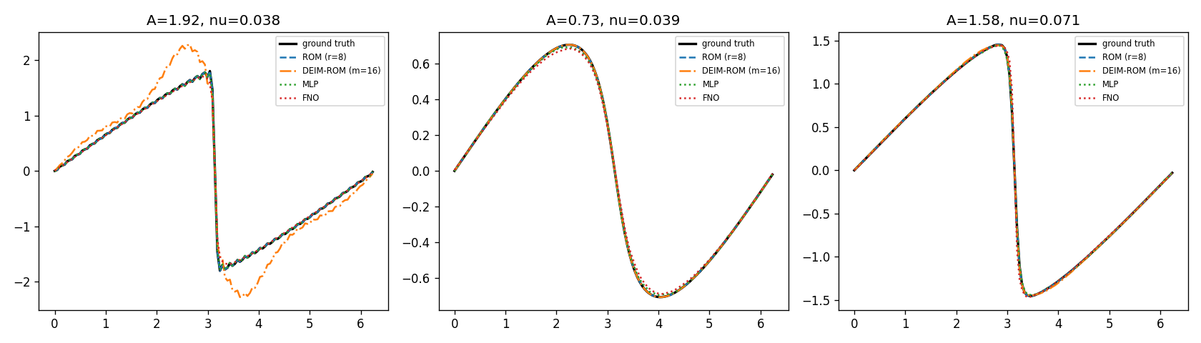
A pseudo-spectral solver generates ground-truth trajectories; a rank-8 POD-Galerkin ROM projects the governing equations onto a low-dimensional basis; a hybrid DEIM/local finite-difference scheme hyper-reduces the ROM's online cost (DEIM's interpolatory projection is exact, but the nonlinear-term value it interpolates is obtained via a local finite-difference surrogate rather than the true spectral evaluation, since the latter is inherently global); and an MLP surrogate and a 1D Fourier Neural Operator learn the map from parameters and from the initial field and viscosity, respectively, to the solution. The full-order solver and four approximations are compared on relative L² error and offline/online cost.
Result
The POD-Galerkin ROM is most accurate in-distribution and generalises best to the unseen family, but it is slower than the full solver. The DEIM/local-finite-difference variant removes the full-grid cost: over 40 test cases its mean error is 4.3% (median 0.24%, up to 53% on steep, low-viscosity cases). Its speed relative to the full solver at the benchmark resolution (Nx = 128) is implementation- and environment-dependent, so no single speed-up is claimed: averaged over the 40 test cases on the same machine, it is 1.6 to 1.9 times faster with NumPy 2.0 and slightly slower (0.8 to 0.9 times) with NumPy 1.26, whose FFT is about three times faster at this size. In a separate two-case scaling check, not a workload average, the advantage grows with resolution: at Nx = 1024, about 2.5 times faster with NumPy 1.26 and 4.1 times with NumPy 2.0. The FNO given the viscosity reaches 0.90% in distribution (5 seeds) but 22.6% on the unseen initial-condition family, so knowing the viscosity does not make it transfer to a new family; the original FNO without the viscosity input reached 2.9% and 23.4%.
Diagnosis
DEIM interpolation itself is accurate (with the exact nonlinear term it matches the plain ROM). The accuracy loss comes from the local finite-difference evaluation: on steep, low-viscosity trajectories the reduced DEIM/local-FD system has positive real Jacobian eigenvalues, a linear instability that a smaller time step does not remove. A higher-order stencil lowered the median error but not the worst cases and cost more online time. Whether broader FNO training distributions or an autoregressive architecture would improve out-of-family generalisation remains an open question, outside this study. This is an empirical accuracy-runtime and generalisation study, not a claim of state-of-the-art or of a general result about any of these methods beyond this specific benchmark.
Limitations
One 1D problem at one training distribution. The plain ROM is slower than the full solver; the DEIM/local-FD variant is unreliable on steep, low-viscosity cases and its speed-up at Nx = 128 depends on the software environment. The FNO results are specific to this network, 200 training trajectories and one initial-condition family.