Inverse problems · Imaging
My contribution
I compared calibrated time-reversal, a learned U-Net refinement and Tikhonov-regularised inversion on synthetic acoustic data, including a multi-network evaluation and a model-mismatch check.
Research implementation
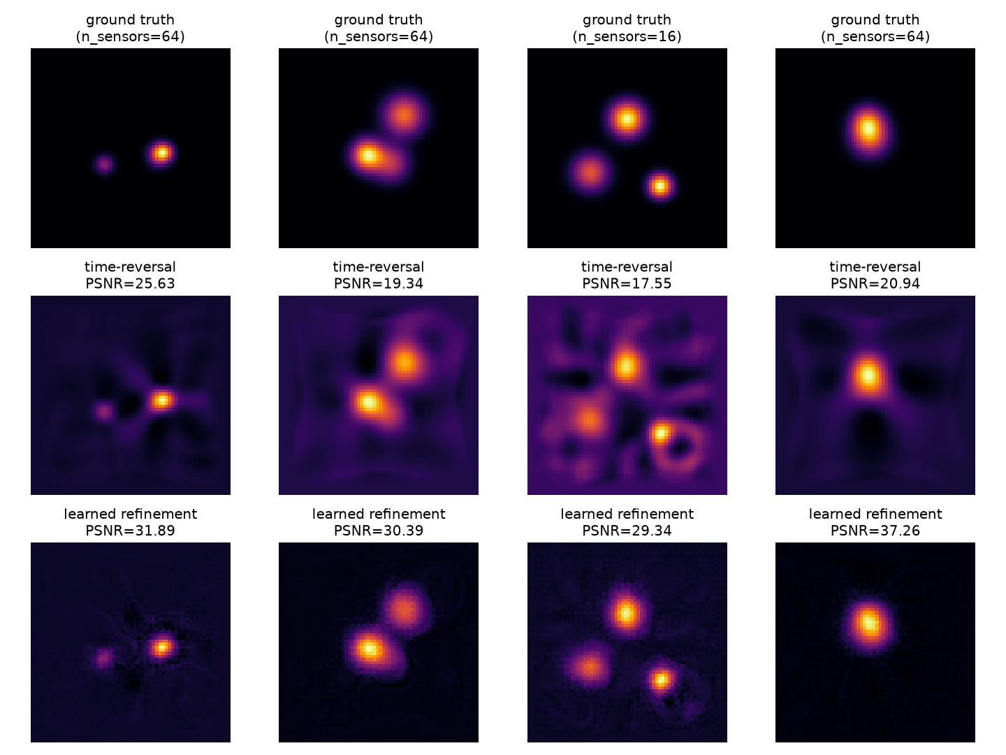
U-Net: +4.9 dB (16 sensors) and +3.2 dB (64) PSNR over calibrated time-reversal on 400 test images; Tikhonov with a noise-matched weight scores higher when the forward model is exact, and its lead shrinks under model error.
Problem
Reconstructing the initial pressure distribution of an imaged structure from sparse-view photoacoustic sensor measurements (a PDE-governed acoustic inverse problem), where classical time-reversal reconstruction degrades into streak artefacts as the sensor array is undersampled.
Approach
A synthetic acoustic forward model (j-Wave) simulates PML-bounded wave propagation from seeded Gaussian-blob phantoms to a sparse circular sensor array (16 or 64 sensors). Three reconstructions are compared: time-reversal, amplitude-calibrated by one least-squares gain per sensor count; a U-Net (adapted from the abdominal-CT-segmentation architecture) that refines the time-reversal estimate; and Tikhonov-regularised least squares through the forward simulator written as an explicit matrix and solved directly. Calibration gains and the Tikhonov weight are fitted on the training split only.
Verification
400 held-out test images (200 per sensor count) and 5 independently trained networks, with 95% bootstrap intervals over images reported separately from the spread between networks. Saved results regenerate exactly and network training is bit-reproducible; the Tikhonov matrix reproduces the simulator, and its adjoint, gradient and normal equations are tested.
Result
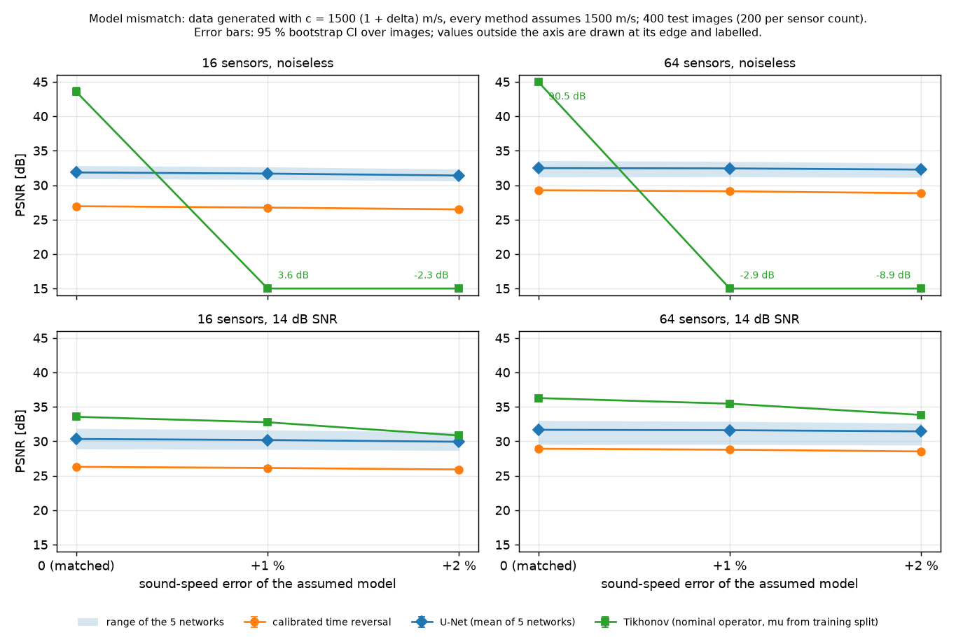
The U-Net improves PSNR over calibrated time-reversal by 4.9 dB at 16 sensors and 3.2 dB at 64, with about 2 dB variation between trained networks; most of the 11 to 12 dB gap to raw time-reversal is amplitude scale. Tikhonov with the exact forward operator and a weight tuned for the known noise level scores higher still (in PSNR at every noise level against the average network, and in SSIM except at 6 dB SNR with 16 sensors, where the two are level), but this is an inverse crime: its noiseless values (43.6 and 90.5 dB) are near-exact inversion of data generated by the same operator.
Model mismatch
With the data generated at a sound speed 1 to 2% above the value every method assumes, Tikhonov tuned on noiseless data fails. At 14 dB SNR, with its weight tuned for that noise level, its PSNR lead over the U-Net shrinks to 0.9 to 3.9 dB, and at 2% with 16 sensors the U-Net is ahead in SSIM. Time-reversal and the U-Net change by under 0.5 dB. The ranking depends on model accuracy, knowledge of the noise level and the metric: in these tests a well-regularised Tikhonov stays ahead of the average network in PSNR; the best single network is ahead at 6 dB SNR and at 2% mismatch with 16 sensors, and Tikhonov's advantage depends on choosing the weight for the actual data errors.
Limitations
Synthetic blob phantoms on a 64 × 64 grid; one mismatch type (sound speed); the U-Net is trained on 40 images and 3 of 5 networks select their final epoch; i.i.d. Gaussian noise only; Tikhonov's weight uses the known test noise level. Whole-image SSIM also penalises a faint background haze in the learned reconstructions.